Description
This example describes how to import and use structural data generated by Rockmass Technologies mapping instrumentation (see https://www.rockmasstech.com).
The example uses actual fracture data that was mapped underground at Kidd mine, Ontario Canada.
Structural Data
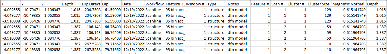
Structural data mapped using Rockmass Technologies instrumentation can be saved in csv format, also used by Leapfrog. The format consists of a header row, followed by the data. Many different data fields may be included or omitted - the importing by 3DEC will read whatever headers and data are in the file. For importing by 3DEC, the file must contain the following headers:
- X
- Y
- Z
- Dip
- Dip Direction
- Feature #
- Window #
An example file showing the first few lines is shown in Figure 1.
3DEC Model - Deterministic
The actual measured features can be imported and DFN fractures can be created. In this case it is assumed that the user wishes to model the individual features as measured. To generate a random distribution of features based on the measured data see the next section.
The measured features can be imported by considering each measurement a single feature, or by averaging the location and orientation for all feature with the same Feature # and Window #. Averaging is the default behavior.
An example command used to import the Kidd data is shown below (the entire data file is shown here).
fracture import from-file 'leapfrog-2022-12-19-1948.csv' format rockmass size 1
Note that a size must be given when importing this data. The size of the features cannot be determined from the data file, so a diameter must be given to enable generation of the disks (fractures) that form the DFN. The resulting fractures from imported with the command are plotted in Figure 2. The scanned tunnel surface for each window is also imported as a DXF and is plotted in the same figure.
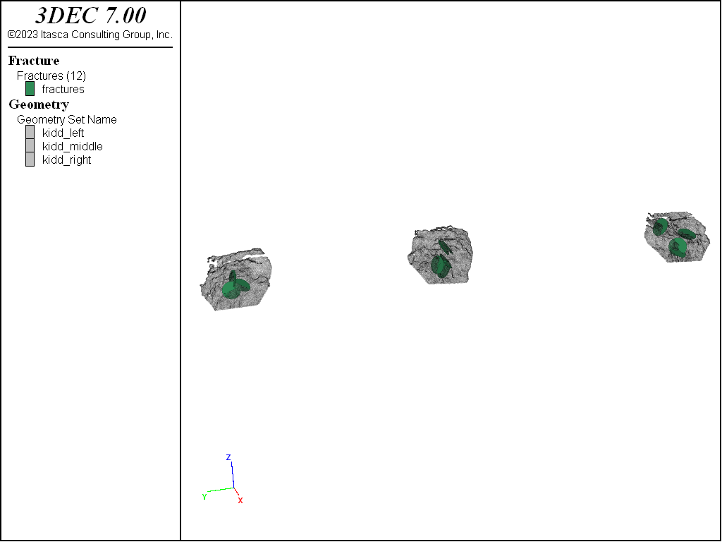
In this figure, the features with the same Window # and Feature # are averaged, so the 81 mapped orientations become 12 DFN fractures. The fractures can be colored by any of the data read from the file. In Figure 2 the fractures are colored by Window #.
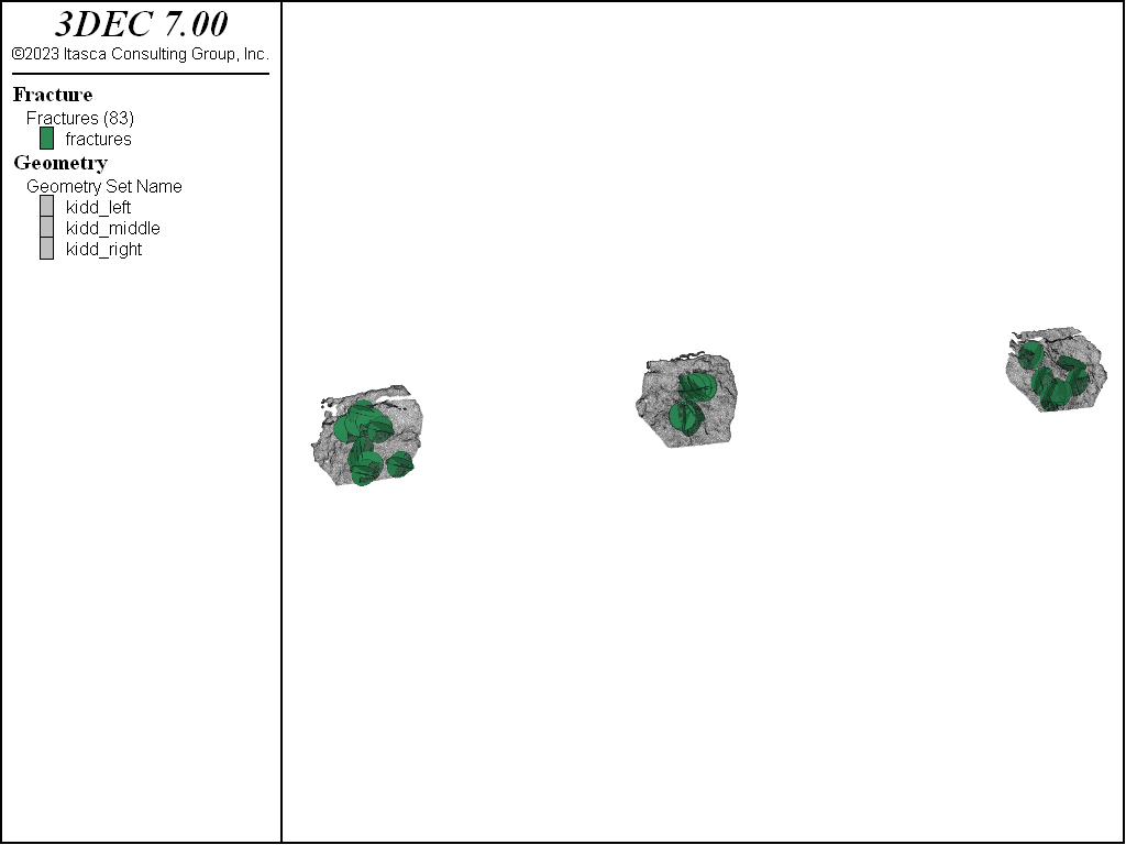
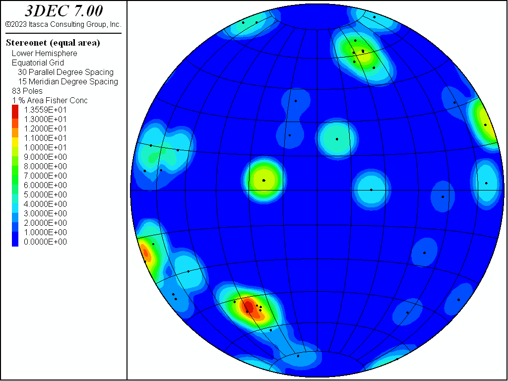
To create a fracture for every measurement, without averaging, add average false to the end of the command above. This yields the fractures shown in Figure 3 (this time colored by Feature #). The stereonet for the 81 fractures is shown in Figure 4.
The imported fractures can now be used to cut faults in a 3DEC model. A simple representation of the actual tunnel is created in 3DEC. A square cross-section is assumed for simplicity. See below for the data file to create the model shown below. For making the model, a fracture diameter of 5 m is assumed, rather than the 1 m diameter shown above. After the model is created, the imported fractures are used to cut the model using the command:
block cut dfn name 'leapfrog-2022-12-19-1948'
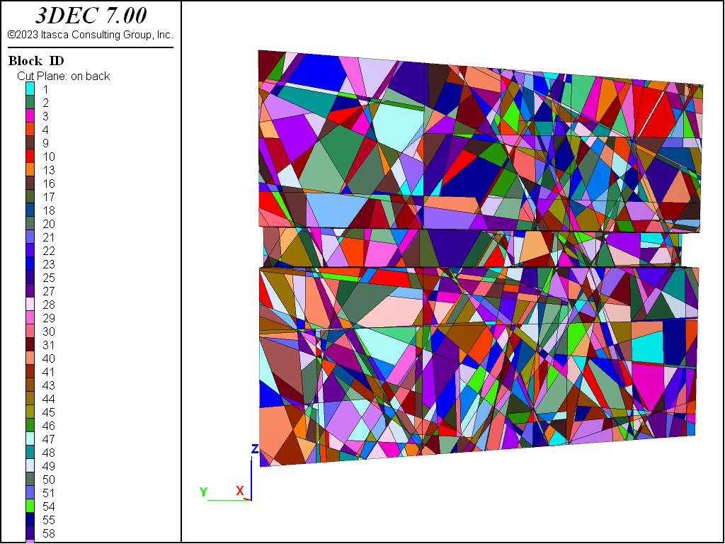
Note that the imported fractures are automatically assigned to a single DFN called ‘leapfrog-2022-12-19-1948’, which is the name of the imported file without the .csv extension. A different DFN name can be set manually when the fractures are imported. The cut model (using the averaged fractures) is shown in Figure 5.
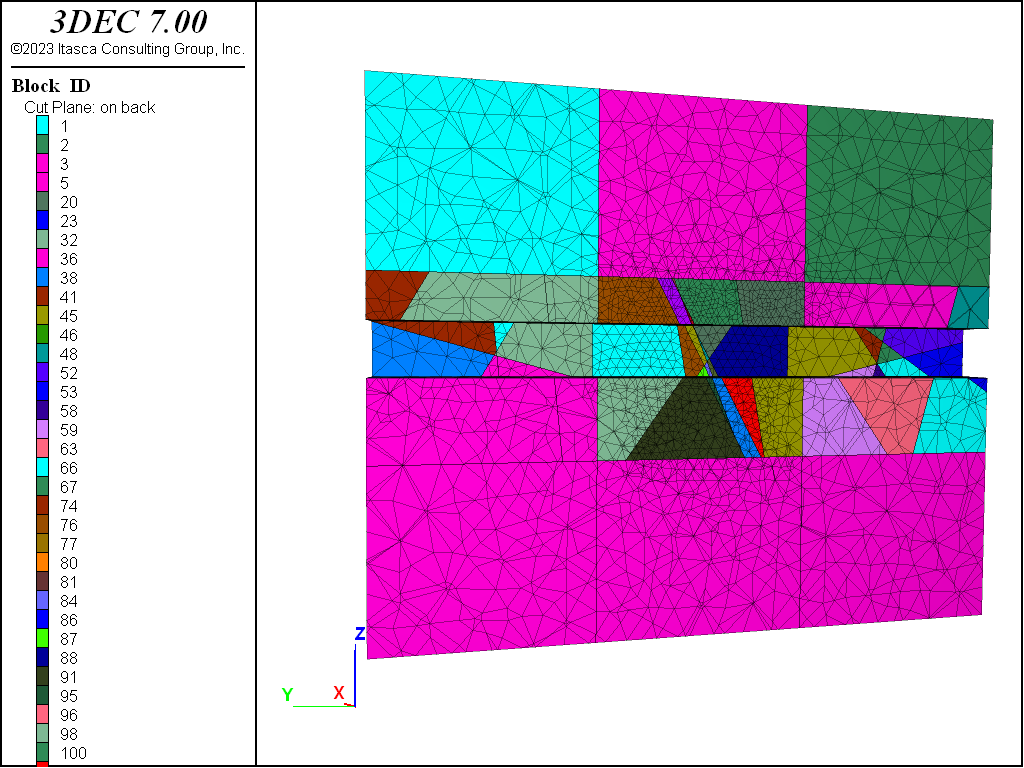
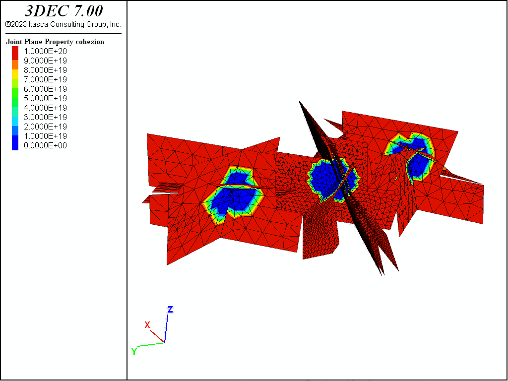
In 3DEC, a cut must slice all the way through a block - you cannot have partially cut blocks. Since the extent of the fractures is unknown, the model shown in Figure 5 may be useful as a worst-case scenario. However, if you want to limit the extent of the fractures, you can assign different properties to the subcontacts inside and outside of the circular fractures. This is done with the command below. This will set a high cohesion outside of the fractures and a zero cohesion within the disks. The same approach can be used for other properties.
block contact property cohesion 1e20
block contact property cohesion 0 range dfn-3dec 'leapfrog-2022-12-19-1948'
3DEC Model - Stochastic
Another way to use the field data is to import the orientations and use these to inform a randomly generated DFN with a large number of fractures. Multiple different DFNs could be created with different randomness but using the same orientation distribution.
The imported Rockmass data can be used to “bootstrap” the randomly generated fracture orientations. Example commands using the Kidd data set are shown below.
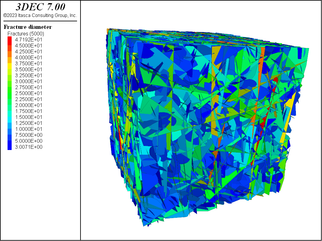
fracture template create 'template1' orientation rockmass 'leapfrog-2022-12-19-1948.csv' size power-law 3 size-limits 5 50
fracture generate template 'template1' fracture-count 5000
In this example, a “template” is created that defines the location, orientation and size distributions. A specific DFN is then created following this template. The DFN is created with 5000 fractures.
The resulting DFN is shown in Figure 7, and the resulting stereonet of orientations is shown in Figure 8. Compare this to Figure 4, which shows the stereonet for the original imported data.

These fractures can then be used to cut a 3DEC model as for the deterministic case above (Figure 9).
Project Files
Download the project files (5 MB, *.zip)
This example is also available in Itasca's online documentation set.
